Excel will display data when double clicking or right-clicking a file and choosing open but can remove some data from the file as it doesn't know the format of the cells.
More options on how Excel displays this data are available when using the built in Text Import Wizard which automatically launches when following the below steps.
Open a CSV in Excel
-
Go to File > Open and browse to the location that contains the CSV file
-
Select All Files in the file type dropdown list in the Open dialog box
-
Locate and double-click the text file that you want to open
-
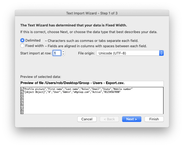
If the file is a CSV file, Excel starts the Import Text Wizard
-
- The Text Import Wizard examines the text file that you are importing and helps you ensure that the data is imported in the way that you want
- Step 1 of 3 is to check Delimited as the file is separated by commas
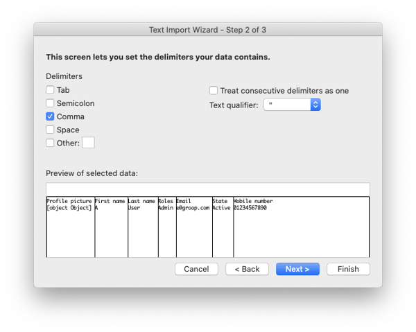
- Step 2 of 3 is to check Comma as this is what identifies separate columns, you will see a preview of the data in the window
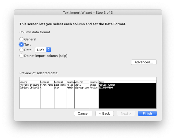
- Step 3 of 3 is to specify which format to apply to each column. eg. choose the column related to a phone number and change the format from General to Text, this will tell Excel to display the cells and retain the leading zero
- Step 1 of 3 is to check Delimited as the file is separated by commas
How to separate Date and Time
- Select the cell or column that contains the text you want to split
- Select Data > Text to Columns
- In the Convert Text to Columns Wizard, select Delimited > Next
- Select the Delimiters for your data. For example Space if you are seperating the time from the date in a Groop CSV. You can see a preview of your data in the Data preview window
- Select Next
- Select the Column data format or use what Excel chose for you
- Select the Destination, which is where you want the split data to appear on your worksheet
- Select Finish
How to format cells as Date
Follow these steps:
- Select the cells you want to format
- Press CTRL+1
- In the Format Cells box, click the Number tab
- In the Category list, click Date

- Under Type, pick a date format. Your format will preview in the Sample box with the first date in your data
Note: Date formats that begin with an asterisk (*) will change if you change the regional date and time settings in Control Panel. Formats without an asterisk won’t change.
If you want to use a date format according to how another language displays dates, choose the language in Locale (location).